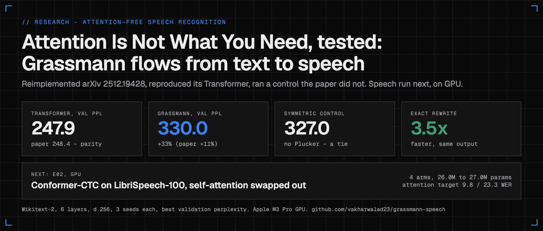
Grassmann flows is the attention-free layer from "Attention Is Not What You Need" (Zhang Chong, arXiv 2512.19428, December 2025). Instead of comparing every token with every other token, it pairs each token with a few earlier ones at fixed offsets, turns each pair into the plane the two vectors span (Plucker coordinates on a Grassmann manifold) and gates that back in. Cost is linear in sequence length. The paper tests it on text only. I wanted to know if it can replace self-attention in attention-free speech recognition, and as far as I could find, nobody has published that test. So I did it in order. First I rebuilt the layer with tests and made it 3.5x faster with an exact rewrite (same output to 1e-12). Then I reproduced the paper's language model setup on my Mac: the Transformer baseline hit 247.9 +- 2.3 perplexity against the paper's 248.4, but the Grassmann model landed at 330.0 +- 0.5, 33% worse, three times the gap the paper reports. The surprise: a same-size control without the Grassmann geometry scored 327.0 +- 2.0, a statistical tie. The geometry is not doing the work. Last, I wrote the speech experiment, a 15-block Conformer-CTC on LibriSpeech-100 with four arms (attention, Grassmann, the symmetric control, no mixer) on two independent code paths. It passes every CPU check and needs about 32 to 64 A100 hours for its first seed, so it runs on a GPU next. The code is public and MIT licensed: github.com/vakharwalad23/grassmann-speech.
Why test an attention-free layer on speech recognition?
Most strong speech recognizers today have self-attention inside them: Whisper, and the Conformer family behind models like Parakeet. I work on on-device speech, and I have written about NVIDIA's Nemotron streaming ASR and building a local dictation app. Attention is the part of those models that grows badly with input length.
Here is why. Self-attention lets every position look at every other position. For a sequence of L frames that is L times L comparisons. Speech is long: after the usual 4x subsampling, a speech encoder sees one frame every 40 ms, so 25 frames per second. A 12.7 second utterance is about 317 frames, and a five minute recording is 7,500. Double the audio and attention does four times the work.
So when a paper titled "Attention Is Not What You Need" claims a layer with no attention at all, linear in sequence length, within 10 to 15 percent of a Transformer, the obvious question for me was: does it work for speech?
Before building the speech test I looked for anyone who had already tried. The search covered GitHub code and repositories, arXiv, Semantic Scholar and OpenAlex citations of the paper, and the title lists of Interspeech 2025 (about 1,179 papers) and Interspeech 2026 (about 1,379 papers). As of 13 November 2026 there was no speech or audio use of this layer anywhere I could reach. The paper's citations at that point (five distinct works across the two indexes) cover LLM sparsity, RNA, patents, an image block and a language architecture. None is audio. That is absence in search, not proof, but it means this is, as far as I can tell, the first public attempt to put this layer into a speech recognizer.
The rule I set for myself from the start: Grassmann against attention only at matched parameters, data, steps and frontend, and only after the attention baseline reproduces a published number. Otherwise any gap could be my training recipe, not the layer.
What does "Attention Is Not What You Need" claim?
The paper is one version, v1, posted 22 December 2025, by a single author, Zhang Chong. Its full title is "Attention Is Not What You Need: Grassmann Flows as an Attention-Free Alternative for Sequence Modeling." There is no code link on the paper, the abstract page or the Hugging Face paper page.
It makes three claims:
- A language model built only from Causal Grassmann layers, at 13 to 18 million parameters, reaches validation perplexity within about 10 to 15 percent of a size-matched Transformer on Wikitext-2.
- A Grassmann classification head on a frozen DistilBERT slightly beats a Transformer head on SNLI: 0.8538 against 0.8511 test accuracy.
- The layer's cost is linear in sequence length.
Here is the paper's Table 1, which is the number I would later try to reproduce:
| Model | Layers | Params | Val PPL |
|---|---|---|---|
| TransformerLM (block size 128) | 6 | 12.59M | 248.4 |
| GrassmannLM (block size 128) | 6 | 13.00M | 275.7 |
| TransformerLM (block size 128) | 6 | 12.59M | 253.6 |
| GrassmannLM (block size 128) | 6 | 13.00M | 282.3 |
275.7 against 248.4 is the "11 percent" gap. The paper does not label the rows by window schedule; the second pair appears to use a different one. A 12-layer pair in Table 2 shows the same ratio: 261.1 against 235.2.
Perplexity, if you have not met it, is the exponential of the average loss per token. A perplexity of 248 means that on average the model is as unsure as if it were picking uniformly among 248 tokens. Lower is better. On Wikitext-2 with a small model and a BERT tokenizer, numbers in the 200s are normal.
The SNLI gap, 0.0027, is about 27 sentence pairs out of roughly 9,800 test pairs. One standard error of accuracy at that size is about 0.0036, so that result reads as a tie.
How does the Causal Grassmann layer work?
Start with the geometry, because it is the whole pitch.
Take two vectors a and b. Together they span a plane: every combination of a and b lies in it. The set of all planes through the origin in r-dimensional space is a manifold called the Grassmannian, written Gr(2, r). Each plane is one point on it.
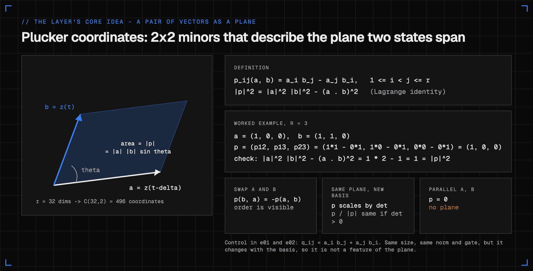
You can describe that plane with numbers using Plucker coordinates: all the 2x2 minors of the pair.
p_ij(a, b) = a_i * b_j - a_j * b_i for every 1 <= i < j <= r
With r = 32 dimensions there are 32 x 31 / 2 = 496 such minors, so each pair becomes a 496-number vector.
These coordinates have properties that make them attractive for a sequence model:
- Order is visible. Swap a and b and every coordinate flips sign: p(b, a) = -p(a, b). The layer can tell "earlier then later" from "later then earlier."
- They describe the plane, not the two vectors. Replace a and b with any other two vectors spanning the same plane and p only scales by the determinant of the change. After normalizing to unit length it is the same vector (for a positive determinant).
- The norm is an area. The length of p is the area of the parallelogram a and b make: the norm of a, times the norm of b, times the sine of the angle between them. If a and b point the same way, p is zero. There is no plane.
The last property has a neat identity behind it, which will matter later for speed:
|p|^2 = |a|^2 * |b|^2 - (a . b)^2 (Lagrange identity)
Worked example: a = (1, 0, 0) and b = (1, 1, 0). The three minors are p12 = 11 - 01 = 1, p13 = 10 - 01 = 0 and p23 = 00 - 01 = 0, so p = (1, 0, 0) and the squared norm is 1. The identity gives 1 x 2 - 1^2 = 1. Same answer from three dot products, without forming any coordinates.
The layer, step by step
The Causal Grassmann block replaces the attention sub-block of a Transformer. At width d = 256:
- Reduce. Project each hidden state h_t from 256 down to r = 32 dimensions: z_t.
- Pair. For each offset delta in the set 1, 2, 4, 8, 12, 16, pair z_t with z_(t-delta).
- Plane. Turn each pair into its 496 Plucker coordinates.
- Normalize. Scale each Plucker vector to unit length (the paper calls this optional; I keep it on, with eps 1e-6).
- Project and average. One shared linear map takes 496 back to 256. Average over the valid offsets: g_t.
- Gate. alpha_t = sigmoid(W_gate [h_t ; g_t]), then mix: alpha_t * h_t + (1 - alpha_t) * g_t.
- Normalize and feed forward. LayerNorm, then the usual 256 -> 1024 -> 256 feed-forward network with a residual and another LayerNorm.
No position ever compares itself with all others. Each sees six partners, so cost grows linearly with length. Stacked over six layers, a token reaches 6 x 16 = 96 positions back.
Parameter for parameter, the block is almost the same size as a Transformer block:
| Part | Shape | Parameters |
|---|---|---|
| W_red | 256 -> 32 | 8,224 |
| W_plu | 496 -> 256 | 127,232 |
| W_gate | 512 -> 256 | 131,328 |
| 2 LayerNorms | 256 | 1,024 |
| FFN | 256 -> 1024 -> 256 | 525,568 |
| Grassmann block | 793,376 | |
| Transformer block (attention, 2 LayerNorms, FFN) | 789,760 |
What did reading the paper closely turn up?
Before writing the layer, the research phase covered the paper's equations, the public reimplementations and the closest work in speech. Four things stood out.
1. The printed layer looks at the future. The equations pair z_t with z_(t+delta), a token to the right, and still call the layer causal. Read literally, a next-token language model would see the token it is supposed to predict. The reported perplexities are not those of a leaking model, so the training code probably used t-delta. Every public reimplementation uses t-delta. I did too, and added a unit test that perturbs future tokens and checks no earlier output moves.
2. The parameter counts do not add up. Building the model exactly from the equations gives 12,607,168 parameters for six layers. The paper reports 13.00M. Both depths are short by about 65,800 parameters per layer, which is exactly d^2 + d = 65,792: one undocumented 256 x 256 linear layer per block. Adding it gives 13,001,920 and 18,156,928, matching the paper's 13.00M and 18.16M to the printed digit. Two independent reimplementations also get 12.61M.
3. The training recipe is almost absent. The paper gives 30 epochs, the batch size and the dataset. It does not give the optimizer, learning rate, schedule, warmup, weight decay, dropout rate, initialization, seeds or number of runs. Each table cell is one number.
4. Reimplementations do not reproduce the gap. This is the one that shaped everything after:
| Reimplementation | Setup | Grassmann vs Transformer |
|---|---|---|
| Infatoshi/grassmann-flows | GPT-2 tokenizer, 6 layers, H100 | 22.6% worse (test PPL) |
| alphaXiv paper-implementations | BERT tokenizer, warmup + cosine, 4 configs | 39.0% to 45.3% worse (computed from their table) |
| kanenorman/grassmann | the paper's config; Transformer 248.7 (paper 248.4) | 43.4% worse (356.6 vs 248.7) |
| youdie006/grassmann | pre-norm, small init, one offset per layer, 12 layers, block 256 | 8.2% better (val PPL) |
All single seed. The pattern across them: the stronger the Transformer baseline, the bigger the gap. And one run shows that norm placement and init can flip the ranking (in its strict post-norm run the Transformer diverged).
There were also smaller open choices: whether every layer uses all six offsets or layer l uses only offset l (the receptive field differs: 96 versus 43 tokens over six layers), what to output where no pair exists, sum versus mean. I fixed each choice in code, wrote it down, and kept both readings of the offsets question as separate arms.
What does attention-free speech recognition already look like?
The closest speech evidence comes from other attention replacements. On LibriSpeech train-clean-100 (100 hours) with CTC and greedy decoding, Miyazaki et al. (arXiv 2406.16808, Table 1) report:
| Encoder | Params | test-clean WER | test-other WER |
|---|---|---|---|
| Conformer | 27.0M | 9.8 | 23.3 |
| E-Branchformer | 26.4M | 9.5 | 22.9 |
| Transformer | 17.3M | 12.8 | 28.1 |
| bidirectional Mamba | 26.3M | 9.1 | 23.5 |
| unidirectional Mamba | 24.2M | 15.7 | 33.6 |
Two lessons. A linear-time mixer can match attention in speech, but only when it can look both ways: unidirectional Mamba is far behind. And the Conformer row (27.0M, 9.8 / 23.3) became my parity target, since it is a plain Conformer, CTC-only, greedy, at the size I wanted.
One more number shaped the design. A 28.8M Conformer-CTC on LibriSpeech is reported at 3.7 / 9.2 in one paper (arXiv 2307.07421) and 4.27 / 11.29 in another (arXiv 2510.18684), under different recipes. The gap is up to 2 points. So only comparisons inside one recipe, on one code path, count.
How did I make the Grassmann layer 3.5x faster without changing its output?
The first version followed the paper exactly, and the first speed test on my Mac's GPU (I call it e00) was bad. On an Apple M3 Pro, one Grassmann block took 0.220 s per training step of 16,384 tokens at length 128, against 0.0445 s for attention. Five times slower. It only caught up at length 4,096.
The paper's form does a lot of redundant work. For each token it builds six separate 496-number Plucker vectors and pushes each one through the 496 -> 256 projection, then averages. Two facts let you collapse that.
First, the projection is affine, so the average can move inside it: the mean of (W p_k + b) equals W (mean of p_k) + b. Second, p is linear in each argument, and all six pairs at position t share the same second vector z_t. So the average can move inside p too:
paper form:   g_t = mean over delta of [ W_plu * p(z_(t-delta), z_t) / n(t,delta) + b ]

anchored:     s_t = mean over delta of [ z_(t-delta) / n(t,delta) ]
              g_t = W_plu * p(s_t, z_t) + b

n(t,delta) = max(|p(z_(t-delta), z_t)|, eps)
One Plucker vector and one projection per token, instead of six. The norms n come from the Lagrange identity above, three dot products each, so no per-pair coordinates are ever formed. A unit test checks the two forms agree to 1e-12 in float64.
My first attempt did only the first half (average, then project). That cut the matrix-multiply FLOPs by about 3x (1.82 to 0.55 MFLOP per token per layer at the paper's sizes) and saved no time at all. The measurements pointed at the reason: the time stayed flat at about 0.22 s across lengths, so it was in the elementwise work of building 496 coordinates times six offsets per token, plus the normalizations, which a FLOP counter does not see. The anchored form removes exactly that work.
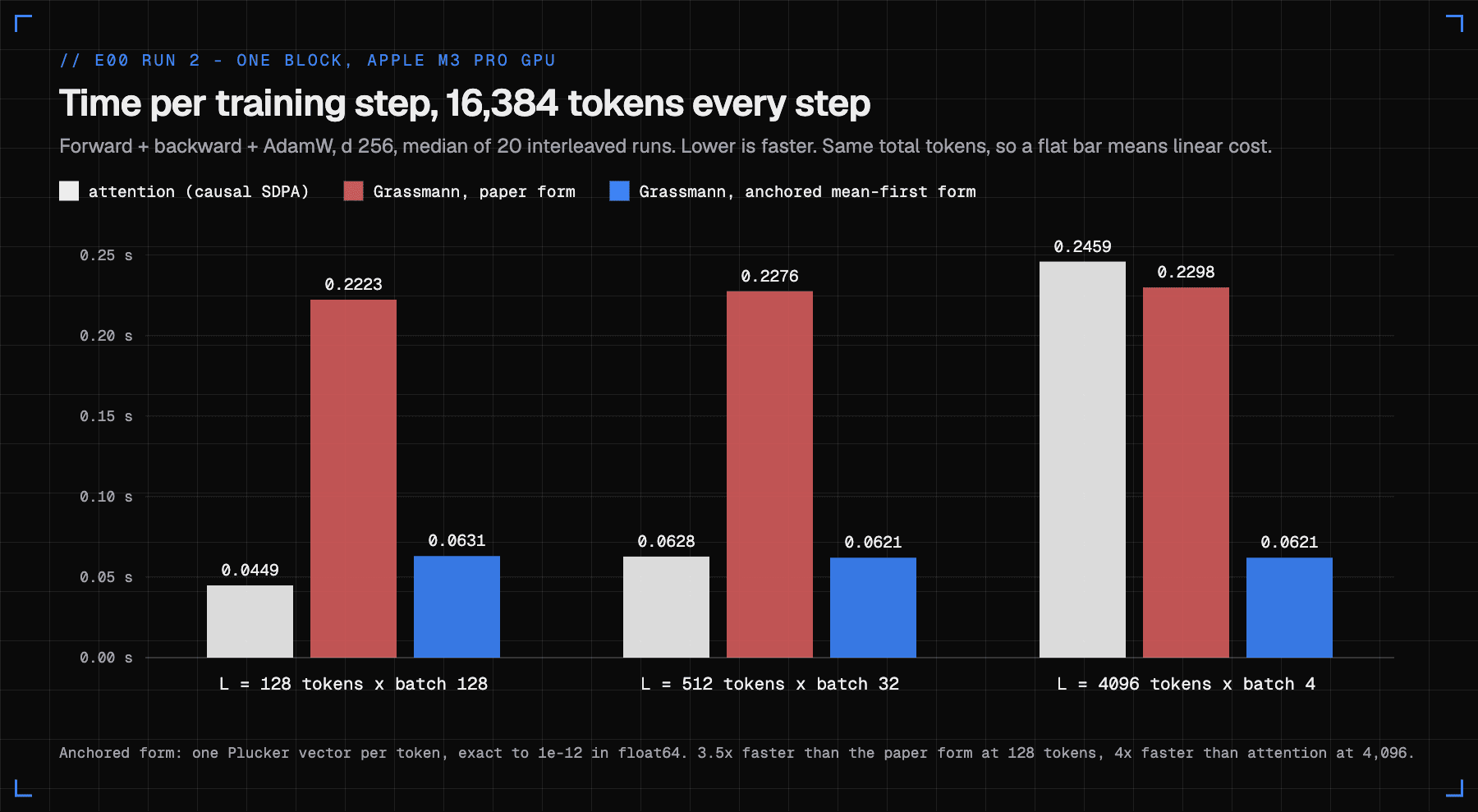
Measured on the same Mac in the second e00 run, same code for the attention control:
| One block, 16,384 tokens per step | Attention | Grassmann, paper form | Grassmann, anchored |
|---|---|---|---|
| L 128 x batch 128 | 0.0449 s | 0.2223 s | 0.0631 s |
| L 512 x batch 32 | 0.0628 s | 0.2276 s | 0.0621 s |
| L 4096 x batch 4 | 0.2459 s | 0.2298 s | 0.0621 s |
The anchored layer is now 3.5x faster than the paper's form at 128 tokens, 1.4x slower than attention there, tied at 512, and 4x faster at 4,096. Its time stays flat while the total token count stays fixed, which is what "linear in length" looks like. The attention control moved under 3.2 percent between the two runs, which bounds the run-to-run drift.
For a whole e01 language model run that meant 0.88 h for Grassmann against 0.76 h for the Transformer, instead of 2 h. It turned a two-night experiment into one night.
Can a laptop train the speech model too?
The same probe timed a full 15-block Conformer-CTC training step (an earlier build: plain attention, no padding) with 16 utterances of 12.7 s each. Attention: 0.852 s in fp32, 0.744 s in bf16. Two-sided Grassmann (the speech variant, below): 0.910 s and 0.903 s. It also checked that PyTorch's CTC loss on the Mac GPU matches the CPU: loss difference 0.0, largest gradient difference 3.9e-6.
The training recipe I wanted to match runs 70 epochs over three speed-perturbed copies of the 100.6 hour training set. The arithmetic:
hours per run = A / (rho * 3600)

A   = 70 epochs x 3 copies x 100.6 h x 3600 s = 7.61e7 audio seconds
rho = audio seconds trained per wall second

attention fp32: rho = 16 x 12.7 / 0.852 = 238.5
                hours = 7.61e7 / (238.5 x 3600) = 88.6 h
77 to 95 hours per run on the Mac. The speech experiment needs four arms, two code paths and ideally three seeds: 24 runs, roughly 1,850 to 2,300 Mac hours (24 x 77 to 95). The language model experiment fits a Mac. The speech experiment does not. The A100 bar is a derived estimate (4 to 8 h per run), not a measurement.
Does the Grassmann layer reproduce the paper? (e01)
e01 is the layer parity test, run entirely on my Mac. Same setup as the paper's Table 1: Wikitext-2, the bert-base-uncased WordPiece tokenizer, blocks of 128 tokens, batch 32, 30 epochs, d 256, six layers, best validation perplexity over training. Four arms:
| Arm | Model | Params | Seeds |
|---|---|---|---|
| transformer | 4 heads, post-LN, causal attention | 12,585,472 | 3 |
| grassmann | all six offsets in every layer (the paper's main reading) | 12,607,168 | 3 |
| control_symmetric | same layer, symmetric products instead of Plucker minors | 12,607,168 | 3 |
| grassmann_one_offset | layer l uses only offset l | 12,607,168 | 1 |
The control is the arm the paper never ran, and I will come back to it.
The first parity attempt failed
The plan was to get the Transformer to the paper's range (validation perplexity 241.0 to 253.6, from the paper's text) before running anything else. If the baseline is weak, a Grassmann model "within 11 percent" means nothing.
Attempt one used the small embedding init most modern language models use, N(0, 0.02), and gradient clipping at 1.0. It ran 0.80 h and gave a best validation perplexity of 1388.4. The training loss sat between 7.29 and 7.18 nats from the first epoch on. I measured the unigram entropy of the training tokens, the loss you get by ignoring the input and predicting word frequencies: 7.190. The model had collapsed into a frequency table.
The model still reacted to its input at initialization, so the collapse happened during training. My best guess (not verified) is that with the output head tied to tiny embedding rows, Adam's steps at learning rate 1e-3 are large compared with the rows, and the shared softmax gradient pulls every row in the same direction.
The fix was to stop inventing a recipe and copy the one that had already reproduced the paper: kanenorman's. That meant PyTorch's default N(0, 1) embedding init, embedding dropout 0.1, no gradient clipping, AdamW at 1e-3 with weight decay 0.01, and a per-epoch cosine schedule. Attempt two: best validation perplexity 247.1 at epoch 20 (test 255.2), against the paper's 248.4 and kanenorman's 248.7. Parity.
The lesson I wrote down: the 0.02 init came from my own quick check, which looked only at the initial loss (about 70 with N(0, 1), which looks alarming). Initial loss was the wrong thing to check.
The sweep
With parity reached, the remaining nine runs went through overnight, 01:27 to 09:37 on 14 November, about 8.2 hours, one after another through a memory guard script that kills a job if the Mac starts swapping hard. Each run takes under an hour; the guard's peak process memory reading was 648 MB.
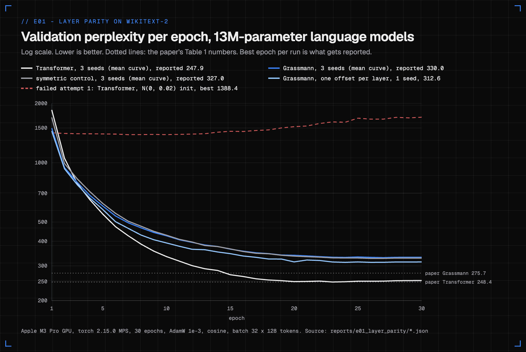
| Arm | Val PPL, seeds 0 / 1 / 2 | Mean +- sd | Test PPL (mean) | vs Transformer |
|---|---|---|---|---|
| transformer | 247.1 / 250.5 / 246.2 | 247.9 +- 2.3 | 260.2 | - |
| grassmann | 329.8 / 329.6 / 330.6 | 330.0 +- 0.5 | 341.5 | +33.1% |
| control_symmetric | 329.3 / 325.6 / 326.2 | 327.0 +- 2.0 | 337.4 | +31.9% |
| grassmann_one_offset | 312.6 | 312.6 (1 seed) | 334.6 | +26.1% |
| paper, Table 1 | 248.4 / 275.7 | - | - | +11.0% |
The Transformer reproduces the paper to 0.2 percent, so the pipeline is trusted. The Grassmann model does not reach 275.7. It lands with the reimplementations, not with the paper.
Is the gap real? The arithmetic
Three seeds per arm is small, so the comparison is done on log perplexity with a t-interval:
Delta = mean(ln PPL_A) - mean(ln PPL_B)
CI95  = Delta +- t(0.975, 2) * sqrt(s_A^2 / n_A + s_B^2 / n_B)

s = per-arm standard deviation of ln PPL, n = 3 seeds, t = 4.303 (2 degrees of freedom)
reported as the ratio exp(Delta)
Worked example, Grassmann against Transformer: Delta = 5.7991 - 5.5132 = 0.2859, standard error 0.0053, interval 0.2631 to 0.3087. As ratios that is 1.301 to 1.362: 30 to 36 percent worse, nowhere near 11.
Grassmann against the symmetric control: Delta = 0.0091, standard error 0.0036, interval -0.0064 to 0.0246, ratio 0.994 to 1.025. The interval contains 1. A tie.
Does the Grassmann geometry matter? The control the paper did not run
This was the most interesting result of the whole project so far.
The symmetric control replaces the Plucker minor a_i b_j - a_j b_i with the symmetric product a_i b_j + a_j b_i. Everything else stays identical: same offsets, same 496 features, same unit normalization (its norm also has a closed form from dot products), same gate, same parameter count, 12,607,168. The only thing it lacks is the geometry. The symmetric feature changes when you pick a different basis for the same plane, so it is not a description of the plane. It is not a point on a Grassmann manifold.
If the Grassmann structure were what made the layer work, the control should be clearly worse. It scored 327.0 against 330.0, a statistical tie, and nominally a little better.
My reading: what the layer learns comes from fixed-offset multiplicative mixing of nearby tokens, not from the Grassmann geometry. Seen as algebra, the Plucker step is a set of antisymmetric bilinear forms between z_t and z_(t-delta). A symmetric bilinear form at the same offsets does as well. That puts the layer in the same family as dilated convolutions and multiplicative interaction layers, with a geometric story on top.
Two more findings from the same sweep:
- The window reading matters more than the geometry. One offset per layer (receptive field 43 tokens) beat all offsets in every layer (96 tokens) by 5 percent: 312.6 against 329.8. That is one seed, so it is not yet a measured difference, but youdie006's reimplementation, the one that beat its Transformer, also used one offset per layer.
- The planes are well defined after training. I logged the sine of the angle between every z_t and its partner. Near initialization the reduced states lined up more and more with depth (median sine 0.99 in the first layer, 0.15 in the last), and thin planes would make the unit normalization amplify noise. After training (seed 0), the median sine is 0.84 to 0.99 in every layer, and at most 0.11 percent of pairs fall below 0.05. Degenerate planes do not explain the gap.
What this does not show: that Grassmann layers are useless. The recipe I used is the Transformer's recipe, tuned for nobody in particular. A Grassmann-specific recipe (pre-norm, warmup) might close part of the gap; youdie006 reports a pre-norm, small-init setup flipping the ranking. I did not test that. What it does show is that any speech result for "Grassmann" alone would not tell you whether the geometry matters. So the speech experiment carries the control too.
How do you put a causal text layer into a speech encoder?
A speech recognizer is not a language model. It hears the whole utterance before it writes the transcript (at least in the offline setting I test first), so there is no reason to forbid looking ahead. And the Mamba numbers above say that looking only backward costs a lot: 15.7 against 9.1 WER on test-clean.
So the speech arm uses a two-sided variant, which is my change and not the paper's method. Each frame t pairs with partners at both t-delta and t+delta, for the same six offsets. Both pairs are ordered (earlier, later), and because Plucker coordinates flip sign when you swap the order, the layer can still tell past from future. The anchored rewrite carries over: the future partners enter the partner sum with a minus sign.
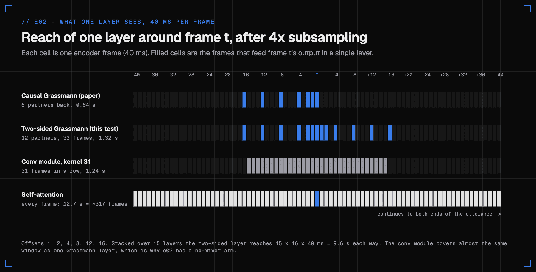
At 40 ms per encoder frame, offset 16 is 0.64 s. One two-sided layer spans 33 frames, 1.32 s. Stacked over 15 layers it reaches 15 x 16 x 40 ms = 9.6 s each way.
That picture also shows the main risk. A Conformer block already has a convolution module with kernel 31, which covers 31 frames, 1.24 s, almost the same window as one Grassmann layer. If the Grassmann mixer only re-learns what the convolution already does, it will look fine against attention and add nothing. So the honest question has two parts: Grassmann against attention, and Grassmann against no mixer at all.
The four arms
The encoder is a 15-block Conformer at width 256, laid out exactly like ESPnet's so the same model runs in two code bases. Only the sequence mixer slot changes.
| Arm | Mixer in each of 15 blocks | Params | vs attention |
|---|---|---|---|
| attention | relative-position multi-head attention, 4 heads | 26,958,472 | - |
| grassmann | two-sided gated Grassmann, r 32, offsets 1 to 16 each side | 26,021,992 | -3.5% |
| symmetric | same with symmetric products (the e01 control) | 26,021,992 | -3.5% |
| no_mixer | none; feed-forward width 1344 instead of 1024 | 26,945,032 | -0.05% |
The Grassmann arms are 3.5 percent smaller, inside my 5 percent matching rule. Every count is a unit test, and a separate check builds the same arms out of ESPnet's own modules and gets the same numbers.
Three engineering details that speech forced
- The gate became a residual branch. Inside a Conformer every sub-block adds onto a residual stream. The Grassmann branch outputs (1 - alpha)(g - u), where u is the LayerNormed input: the paper's blend alpha u + (1 - alpha) g minus u. With alpha = 1 the branch adds nothing, the same way a closed gate behaves in the paper's block.
- Padding. Speech batches mix utterances of different lengths, padded with zeros. A pair counts only when both frames are real, so real frames get exactly the output they would get unpadded (a unit test checks it), and padded frames get a zero Grassmann feature.
- The pair features stay in fp32. Under bf16 mixed precision, the Lagrange norm |a|^2 |b|^2 - (a . b)^2 subtracts two nearly equal numbers and cancels to garbage; in fp16, |z|^4 overflows. The rest of the model runs in mixed precision; the Grassmann pair math does not.
What is the e02 plan on the GPU?
e02 is the speech experiment. The question it answers: does the two-sided Grassmann mixer replace self-attention in a 15 x 256 Conformer-CTC on LibriSpeech-100 at matched size, and does its Plucker structure beat the same-size symmetric control?
My hypothesis, written down before any run: attention reaches about 9.8 / 23.3. The Grassmann arm lands between attention and no mixer, closer to no mixer, because the convolution already covers plus or minus 15 frames and e01 found the geometry adds nothing over the control. I would be happy to be wrong.
Two independent code paths
The same four arms run twice:
- The ESPnet track. ESPnet's own LibriSpeech-100 recipe, pinned at release v.202611, which is the recipe family that produced the published number. My encoders are registered into ESPnet at runtime by a small launcher, so ESPnet itself stays unpatched. This track carries the parity run.
- My own trainer. The same recipe rebuilt in plain PyTorch with my layer code. A second measurement of the same comparison. If the two tracks disagree, that is a finding about a trainer, not the layer.
Both tracks score with one shared WER scorer. On CPU, the two tracks agree on every arm's parameter count, and my log-mel features are within 4.8e-7 of ESPnet's frontend.
| Setting | Value |
|---|---|
| Data | LibriSpeech train-clean-100, speed perturbation 0.9 / 1.0 / 1.1, utterances over 30 s dropped |
| Features | 80 log-mel, 25 ms window, 10 ms hop, global mean and variance normalization |
| SpecAugment | time warp 5, 2 frequency masks up to 27 bins, 5 time masks up to 5% |
| Tokens | unigram SentencePiece, 5000 |
| Optimizer | Adam 2e-3, weight decay 1e-6, 15k warmup steps, gradient clip 5 |
| Training | 70 epochs, average of the 10 best checkpoints |
| Decoding | CTC greedy, no language model |
| Score | WER and CER with error counts on dev-clean, dev-other, test-clean, test-other |
The learning rate follows ESPnet's warmup schedule, which peaks at step 15,000 and then decays as one over the square root of the step:
lr(k) = 2e-3 * 15000^0.5 * min(k^-0.5, k * 15000^-1.5)

k = 7,500:   2e-3 * 15000^0.5 * 7500 * 15000^-1.5 = 2e-3 * 0.5 = 1e-3
k = 60,000:  2e-3 * (15000 / 60000)^0.5          = 1e-3
The run order has a gate
Nothing Grassmann runs until attention reproduces the published number. The parity target is the Miyazaki Conformer at 9.8 test-clean and 23.3 test-other. One caveat: that paper does not publish its encoder config. I inferred 15 blocks at width 256 from the 27.0M parameter count (my build gives 26.96M). If parity misses, the fallback anchor is the recipe's own E-Branchformer, 9.6 / 23.1 in ESPnet's README, which Miyazaki reproduced at 9.5 / 22.9.
Differences between arms get a paired bootstrap over speakers: resample speakers with replacement 1,000 times, recompute the WER difference each time, and take the 2.5 and 97.5 percentiles. An interval that holds zero is a tie, and I will call it one.
What it costs
From a FLOP-based compute estimate, one run is about 4 to 8 hours on an A100 (derived from FLOPs and an assumed utilization; ESPnet's older LibriSpeech-100 Conformer recipe, a joint CTC and attention model, is reported at 15.9 h on one V100-32GB). The recipe's batch size needs a 40 GB or larger card.
- Seed 0, both tracks, four arms: 8 runs, about 32 to 64 A100 hours.
- All three seeds: 24 runs, about 96 to 192 A100 hours.
That is the next step. I am arranging the GPU time now.
What already passed on CPU
Nothing has touched real speech data yet, but every code path has run:
- 63 unit checks: Plucker identities, causality, receptive field, the anchored form's exactness, parameter formulas against ESPnet, padding invariance for every arm, the fp32 mix under bf16, the mel scale, batching, the scorer and the bootstrap.
- A full pipeline on a synthetic corpus: every arm through prepare, train, checkpoint averaging, decode and scoring in 9 seconds. A longer 60-epoch synthetic run took training loss from 87 to 6, so the pipeline learns. (Synthetic held-out WER moved from 100 to about 80 for both attention and Grassmann. That is a smoke test, not a result.)
- The ESPnet track end to end: each arm trains one epoch through ESPnet's own training entry point and decodes through its inference entry point, in 135 seconds on CPU.
What is in the public grassmann-speech repo?
Everything above is in github.com/vakharwalad23/grassmann-speech, MIT licensed. The main branch holds the layer, the language models, the e00 speed probe and the e01 parity experiment with 32 unit checks. The speech code (both e02 tracks, features, LibriSpeech handling, the scorer, 63 checks) sits on the experiments/asr-ctc branch until the GPU results are in.
git clone https://github.com/vakharwalad23/grassmann-speech
cd grassmann-speech
make setup        # python/.venv from the lock file (uv, torch 2.15.0)
make test         # unit checks on CPU, about 5 s
make e01-parity   # Transformer seed 0, ~0.8 h on an M3 Pro; expect val PPL near 248
make e01          # the full sweep, 10 runs, ~9 h on an M3 Pro, resumable
make probe        # e00 speed probe on an Apple GPU, a few minutes, AC power
The pieces worth reading if you want to reuse the layer:
| File | What it holds |
|---|---|
python/src/grassmann_speech/plucker.py | Plucker coordinates, symmetric products, norms from dot products |
python/src/grassmann_speech/mixer.py | GrassmannMixer: causal or two-sided, paper form or anchored, Plucker or symmetric |
python/src/grassmann_speech/blocks.py | the Grassmann block and the post-LN Transformer block |
python/src/grassmann_speech/conformer.py | Conformer-CTC with a mixer slot (the ESPnet-matched arms are on experiments/asr-ctc) |
docs/math.md | every formula with a worked example, including the proof that the anchored form is exact |
Runs pick CUDA, then the Mac GPU, then CPU, and every run report stores the commit, the device and the package versions next to its numbers.
What is the honest status?
| Claim | Status |
|---|---|
| Transformer reproduces the paper's 248.4 (247.9 +- 2.3, 3 seeds) | Measured, Mac GPU |
| Grassmann is 33% worse than the Transformer, CI 30 to 36% | Measured, 3 seeds each |
| Plucker geometry ties a symmetric control (ratio CI 0.994 to 1.025) | Measured, 3 seeds each |
| One offset per layer beats all offsets (312.6 vs 330.0) | One seed; not yet a measured difference |
| Anchored form is exact and 3.5x faster at 128 tokens | Measured (exactness in float64, speed on the Mac GPU) |
| A Grassmann-specific recipe could narrow the gap | Untested |
| Any speech WER for any arm | Not run yet. Code passes CPU checks; GPU next |
| 4 to 8 A100 hours per speech run | Derived estimate, not measured |
| No published speech use of this layer | Searched, none found as of 13 November 2026; absence in search, not proof |
FAQ
What are Grassmann flows in "Attention Is Not What You Need"?
An attention-free layer from arXiv 2512.19428. It reduces each token to 32 dimensions, pairs it with tokens at fixed offsets (1, 2, 4, 8, 12, 16), encodes each pair as the Plucker coordinates of the plane the two vectors span, averages, and gates the result back into the hidden state. Its cost is linear in sequence length.
Does the Grassmann layer match a Transformer on language modeling?
Not in my reproduction. With a Transformer baseline that matches the paper (247.9 against 248.4 validation perplexity), the Grassmann model reached 330.0, 33 percent worse, against the 11 percent the paper reports. Public reimplementations found 22 to 45 percent.
Does the Grassmann geometry matter?
In my language model test, no. A same-size control that swaps the Plucker minors for symmetric products, which are not a function of the plane, scored 327.0 against 330.0. The 95 percent interval for the ratio, 0.994 to 1.025, contains 1, so it is a tie.
Has anyone tested Grassmann flows for speech recognition?
As of 13 November 2026 I found no public code, paper or proceedings title that applies this layer to speech or audio. My e02 experiment, a Conformer-CTC on LibriSpeech-100 with attention, Grassmann, a symmetric control and no mixer, is written and checked on CPU and runs on a GPU next.
Is the code available?
Yes, MIT licensed at github.com/vakharwalad23/grassmann-speech. The layer and the language model experiments are on main; the speech experiment code is on the experiments/asr-ctc branch.
Three things carry over beyond this one layer. First, reproduce the baseline before you trust a gap: my Transformer had to hit 248.4 before the Grassmann number meant anything, and the first attempt collapsed to a word-frequency table. Second, run the control the paper skipped: a symmetric product with the same size, offsets and gate ties the Grassmann layer, so the geometry is a story, and fixed-offset multiplicative mixing is what does the work. Third, an exact rewrite can beat a clever kernel: moving one average inside a bilinear map made the layer 3.5x faster with identical output. The speech test is the open question, and it now has the right arms: attention, Grassmann, the symmetric control and no mixer at all, on two code paths, gated on attention reproducing 9.8 / 23.3. I will publish the WER numbers, whichever way they land.
References
- Attention Is Not What You Need: Grassmann Flows as an Attention-Free Alternative for Sequence Modeling (Zhang Chong, arXiv 2512.19428), and the HTML version
- grassmann-speech: my reimplementation, e00 and e01 experiments, and the e02 speech code (MIT)
- kanenorman/grassmann: the reimplementation whose recipe reproduced the paper's Transformer
- Infatoshi/grassmann-flows
- alphaXiv paper-implementations, attention_is_not_all_you_need
- youdie006/grassmann
- Exploring the Capability of Mamba in Speech Applications (Miyazaki et al., arXiv 2406.16808), the source of the 9.8 / 23.3 Conformer parity target
- Conformer: Convolution-augmented Transformer for Speech Recognition (Gulati et al., arXiv 2005.08100)
- arXiv 2307.07421 and arXiv 2510.18684, the two reports of the same Conformer-CTC size with different WER
- ESPnet LibriSpeech-100 ASR recipe
- LibriSpeech on OpenSLR (CC BY 4.0)
- Wikitext-2 on the Hugging Face Hub
- My earlier speech posts: NVIDIA Nemotron ASR streaming explained, Building TapTalk, local speech to text on macOS, Speculative listening and on-device ASR